


Some time ago, I had to evaluate the transmitted optical power of different samples of communication LEDs. These are special devices with a bandwidth of about 100 MHz, many orders of magnitude faster that general purpose lighting LEDs. To do that, I had to connect a current source to the the light emitter, wait for a while and then measure the optical power at the end of an optical fibre. However, I began to think that was something annoying in this measurement. Something sparkled in my mind: maybe despite the long time I waited to take the measurement, this time was not enough. I was well aware of the fact that these LEDs have quite strong dependency of emitted light vs temperature. The only way to solve this doubt was by measuring the time response of the device.
I just connected an optical to electrical transceiver to a multimeter which was remotely monitored. I captured the tuples of time and voltage and then I plotted them. The result was astonishing, so I processed the data to be sure that I was not committing a mistake but the result was very clear. The response perfectly matched a first order response and the time constant was THREE HUNDRED SECONDS (5 MIN!). I have a clear image in my mind that this was what I wrote in my notebook using capital letters.
The immediate consequence of that if I wanted to measure an stable optical power, I had to wait for at least five time constants: at least 25 minutes until the level had been settled to almost its final steady state. Strictly speaking, is an small fraction of it with just a mere 0.7 % error. Needless to say, I had to repeat all my previous measurements because they were useless. The time I waited was proven to be too short.
Depending on the required precision you may wait less or require more, but first, you need to know if it is a first order one and which is the time constant of your system.

In this post of today I would like to make some comments about the uniqueness of time response of first order systems and to show with an example how to calculate main parameters and also to check if a system really behaves as first order one.
First order system: an electrical example
For electronic engineers, one of the best examples of a first order system is the one of the discharge of a capacitor across a resistor. We will use it because of the beauty of its simplicity.
In this figure, you use the switch to instantly charge the capacitor across a voltage source. Then you switch to the right to discharge it across a resistor.
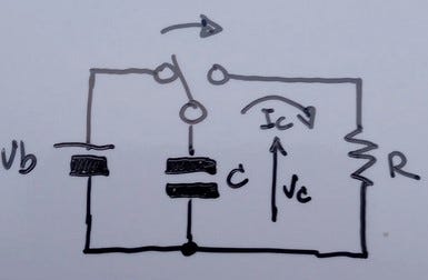
Once the switch is in the right position, the initial current across the resistor and capacitor is predicted by Ohm's law
By the definition of capacitance as the ratio of charge to voltage, the discharge rate will have an initial rate of:
If discharge current where constant, the capacitor would be fully discharged after
However, the discharge current is not constant because as voltage over capacitor decreases, so does the discharge current thus producing a situation in which the capacitor discharges endlessly with an ever decreasing current.
If we apply differential calculus1 we come to a very simple and beautiful expression:
We call time constant (τ) to the R·C product, which has dimensions of time (s).
There are many ways we can visually calculate the time constant if we see an exponential decay:
Time constant is the time it gets the initial slope to cross the steady state.
The time that the signal takes to reach half of the steady state is 0.7 time constants.
When passed time is one time constant, the signal is at 37% of its final value.

The most general response of a first order system to an step is the expression that follows:
A real example of extraction of the time constant
I have done an experiment to extract the time constant of a system.
The experiment consists in a ceramic cup (the one I use to drink tea) that is filled with water, place in a microwave oven, heated and then placed over a support in which there is a thermocouple that records the evolution of temperature. This data will be analyzed with an Octave (GNU octave) script. It is likely to work directly also in Matlab.
Follows raw data plot.
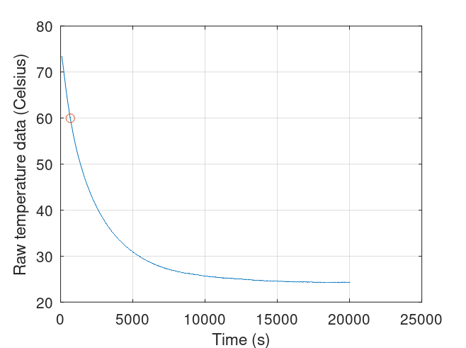
I will analyze data starting from 60 ºC, once the initial transient has settled: the system formed by the thermocouple and the holder.
The first thing that the script does is to normalize the measurement data, removing steady state offset and normalizing the initial value to unity.

Then, the script calculates the logarithm of the data (which is expected to be a line) and calculates its slope by using minimum square error. The slope is the time constant. It is better to use only that part of the measurements in which the signal is strong (in the linear scale). In this example I have taken the data when the normalized temperature is over half of the steady state. This range is plot in red in the following figure (although barely seen).

Time constant (τ) is about 2300 s, 38 minutes. In order to reach an steady state, we have to wait for 5 times (τ), 11700 s. We have waited for 19000 s, which is about 8 time constants.
Now it is time to see how good the fit is, or said in other words, if the measured system really behaves as a first order one or not.

In this example, the fitting is not better because probably the room temperature has drop about one degree (air conditioning?) while doing the long measurement, reducing the settling value. I say so because I manually configure settling value and indeed, the fitting was significantly better. The time constant calculation changes from 2300 to 2200 s (5 % difference).
For an example, it is good enough. If this were a real measurement, it should be repeated. Did you know that measuring right is very difficult?

Funny facts
You can calculate the time constant starting at any point of the decay, but you need to know the settling point. Without it, you cannot calculate it. However, in a system like ours, we know that the settling value will be the ambient temperature. However, measuring it with high precision is not an easy task.
Summary and conclusions
First order systems are widely found in nature and in many cases, knowing the amount of time constant can be of a great help.
Experience also shows that the thermal time constant may be much greater than you can initially think.
Differential calculus was discovered by Isaac Newton between 1665 and 1666 when we has confined in his family house in the fields of Woolsthorpe during the bubonic plague that devastated London at that time. There was no TikTok at that time and this helped.