


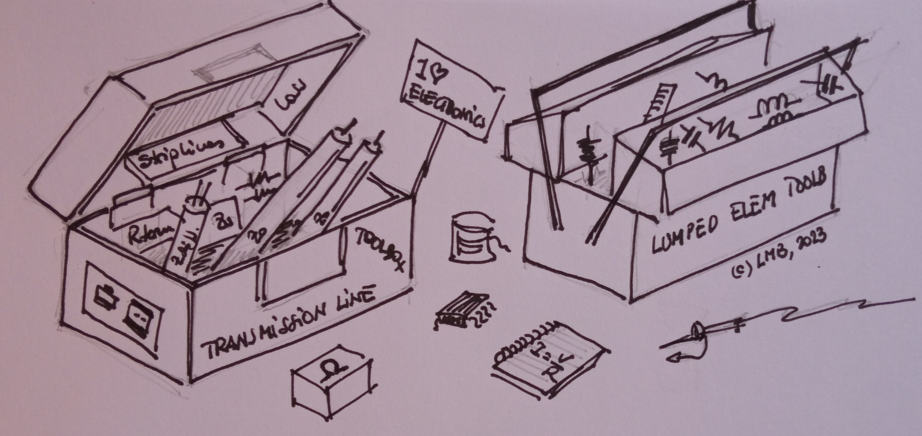
Signal Integrity: a tale of two toolboxes
Does my system require Signal Integrity considerations?

When I start a digital board design, one of the first thing I do is to calculate which nets require the special treatment of high speed lines. This includes also the possible cabling between boards.

If the board is short (relative to signals it carries) we can use the well know Ohm's Law, discrete elements like capacitors, inductors, resistors, semiconductor models… But if the board is long, that is, the time that the signal needs to propagate from source to destination is in the order of the time of a logical level transition, we have to use another tool. One that contains different forms of transmission lines, termination techniques and much more simulation support.
We need to use transmission line models when the end to end propagation delay is longer that an small fraction (say one sixth) of the one that the digital signal needs to change state.
There are two factors involved: transition time and propagation delay. Let us see them one by one.
Propagation delay
The question of how long takes a signal to propagate from origin to destination can be better expressed in terms of how long the electromagnetic field takes to propagate across a medium.
When we work with cables, the manufacturer typically reports the delay per unit length, but some times offers the velocity of propagation compared to light speed. For example, a velocity of 77 % corresponds to a delay of 4.3 ns/m, because light speed in vacuum1 is 3E8 m/s.
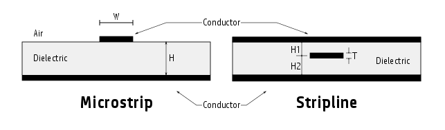
When we have to analyze traces in a PCB, the propagation delay depends on the structure we use. If we use a microstrip, part of the field propagates across air and part across the dielectric. In an stripline, all the field propagates across the dielectric, and results in a greater delay figure.
In a more formal way, delay can be expressed as:
where c is light speed in vacuum and εeff is the effective dielectric constant (dielectric permittivity), a unit-less figure. It is expressed as a ratio with the electric permittivity of vacuum and is always equal or greater than 1.0.
Follows a table that contains approximate data. As I have very poor memory, I am able to memorize figures with just one digit :-). For back of the envelope calculations, is enough.

However, when we need to do more precise calculations (I typically do), we can follow two possible approaches:
Follow IPC-2141A approximation formulas. A nice tool that does that in a very intuitive way can be found in the following link: https://saturnpcb.com/saturn-pcb-toolkit/. It is a very valuable program that include this and other daily use calculations.
Use a 2D field Maxwell equation's solver. There are many tools that support them, most of them commercial (pay). However, I have recently discovered a free online solver (no SW installation required). I have compared results against commercial tools and so far, it has provided fairly accurate results. It is the Sierra Circuits/ProtoExpress calculator. Can be reached in this link https://www.protoexpress.com/tools/pcb-impedance-calculator/
Transition time
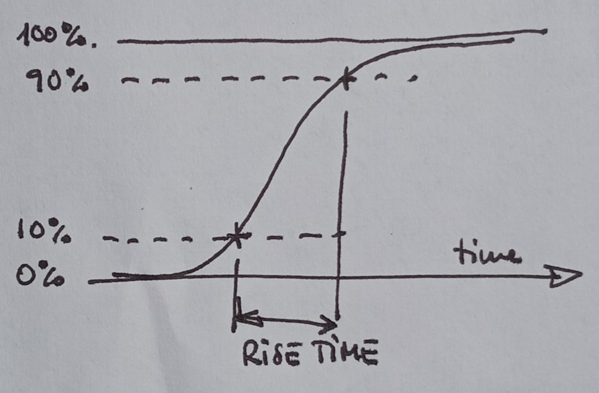
Transition time is the time a digital signal takes to change state. However, we use frequently the term Rise Time (RT), which we assume to be equal to the Fall Time of a signal. If they are not the same, we use the faster of them.
As general agreement, we measure Rise Time as the time the signal takes to go from 10 % of the value to the 90% of the value. If you instruct your oscilloscope to measure rise time, it will use this standard.
To know the rise time of the signals of our circuit we have two main approaches: measurement or datasheet, but there are some times in which we may get the answer by simulation or analytically.
If you decide to measure, you have to be sure that the equipment bandwidth you are using (the oscilloscope and the probe) is not limiting the actual signal rise time. You also need to be careful in measuring correctly. There will be monographic post in this newsletter about this. Take into account that is very likely that the signal bandwidth is large.
The relationship between Rise Time and bandwidth is
For example, a signal with a rise time of 1 ns has an approximate bandwidth of 350 MHz. If you measure a rise time whose equivalent bandwidth is similar to oscilloscope or probe, be suspicious about precision.
Spacial extend of an edge
If we combine transition time and propagation delay per unit length, we obtain the distance that an edge requires to propagate.
If the physical distance of your circuit is longer than L/6 , we need to use transmission line models. If lower, a lumped element model is good enough.
In the next week’s newsletter we will work with real examples of the theory examined today.
The light speed in air is (for engineering accuracy) the same than over vacuum.