


QucsStudio evaluation and transmission line mismatch (2)
Tool evaluation continues with more interesting features and the first s-parameters tricks are introduced

PCB transmission lines
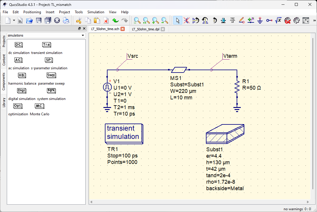
The next step in the QucsStudio exploration will be a transmission line made of PCB and defined by geometrical parameters.
QucsStudio does it in a very elegant way: you have to include a) substrate information and b) the geometrical specification of transmission line that makes reference to the PCB substrate. According to manual, in this state, QucsStudio makes theoretical calculations based on approximated formulas, does not use an electromagnetic solver.

I will add:
a substrate.
a microstrip line
I will fill in the geometrical parameters with data taken from a real 8-layer PCB:
Microstrip line of 50 Ω characteristic impedance.
Copper thickness: 17 μm of copper base plus 25 μm electroplated, results in 42 μm.
Dielectric based of FR-4 with a dielectric constant (DK) of 4.4 and a thickness of 130 μm. We are not interested in high frequency losses and we will not complicate the model with more parameters.
No coating, a model limitation. We found in a previous article that coating introduces significant effect.
Trace width of 220 μm (calculated for target characteristic impedance with an external tool).
Trace length: 10 mm (arbitrary decision).
S-parameter refresh
As we are dealing with high speed digital design, we are going to do a fast refresh of scattering parameters (s-parameters) used for modeling linear systems. For a single ended system, two of them are the most relevant to us.
s21: ratio of he voltage that reaches the port 2 (the output) related to the one that we have in port 1 (the input). The nomenclature could sound the inverse one of the expected. This is the transfer function (or gain) we have always evaluated in electronics.
s11: the input signal that is reflected back to the source: we know that when there is a mismatch, signal is reflected, but many people does not know that in a passive filter, in the attenuation band the energy of the signal is not vanished in the void but reflected back to the source (an typically dissipated in the form of heat).
Simulation and fun
When I simulate it, the fun starts because non ideal systems tend to behave non ideally and this is an opportunity to learn.

I have displayed in different graphs the transmission parameters (s21) and reflection ones (s11). I see:
There is a negligible amount of transmission losses, due to skin effect and limited conductivity in the copper. Transmission line is no more ideal.
The more challenging fact comes from the reflection loss. The transmission line impedance is quite close to 50 Ω (calculations are correct) but it is not exactly equal to this value, which means that there will be some reflections: very small amount of them. A s11 parameter of -45 dB is really very small amount of mismatch. An amount of less that 13 dB is negligible.
Theory predicts that the ripple will have the periodicity of a quarter wavelength (λ/4). Transmission speed is described by the following formula.
The field propagates over the dielectric and over the air. The effective dielectric constant is lower than the dielectric (the FR4, set to 4.4). We will see that the difference between them is about 20 %.
Calculating propagation delay
To calculate propagation delay I will create another circuit and do a transient simulation. I will also set some net labels to allow display transient simulation.
The result is in the following figure.
I have used extensively the ‘Equation’ capabilities (the last option in the 'diagrams' components) to calculate the effective dielectric constant and the frequency of quarter wavelength (Flo4). [The ‘Equation’ option is really nice once you understand its dynamics). In this time the result is 4.17 GHz, which departs only 3 % of the previous notch calculation, a difference that is probably due just to resolution of simulation frequency sweep.

Transmission line impedance
We have seen in a previous step that the reflection coefficient (s11) can allow us to calculate the impedance of the line, and I included the formula to get it and also the QucsStudio function to get it (rtoz(s11(f), [Z0 ref]). One could expect to get a flat value, but instead of that, we are getting a sinusoid. The ripple is low but if the mismatch is greater, it will rise.

It worth stopping for a while to get a deeper understanding of the transformation and its graphical representation.
What the transformation gives us is the impedance seen by the generator across frequency of the combination of the transmission line and the termination. If both are equal, no problem: we will get flat response, but this is not our situation.
Let us see what happens when the transmission line has a characteristic impedance of 60 Ω but is terminated with 50 Ω.
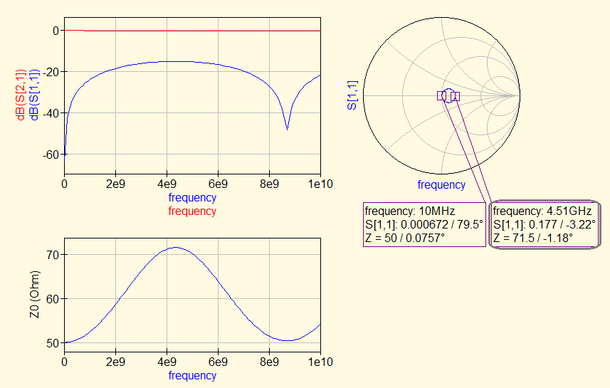
At DC, the transmission line is just a trace of copper with low resistivity. The generator will just see the terminator: 50 Ω.
At quarter wavelength frequency, (about 4.3 GHz) the round trip delay is half wavelength. The reflected signal is in counterphase to the incident one and in the generator current is less: this appears to increase impedance seen by the circuit combination. The mismatch is maximum.
At half wavelength frequency (about 8.7 GHz) the round trip delay produces a reflected signal in the generator that is in phase with the incident one.
Precisely because of that, measuring transmission line impedance by using s-parameters is not easy for the naked eye.
Two alternative approaches can be used:
de-embed the frequency response using mathematical transformations, or
use the much more powerful time domain analysis, that can display how impedance evolves across propagation time.
There are instruments that does such a measurement. They are called Time Domain Reflectometer (TDR) and can be implemented using time-domain techniques (which implies a very sharp square generator and a very fast sampler) or frequency-domain techniques.
However, any simulator can be instructed to display impedance across time: simulator allow to get data that in a real instrument would be very difficult to measure with precision.
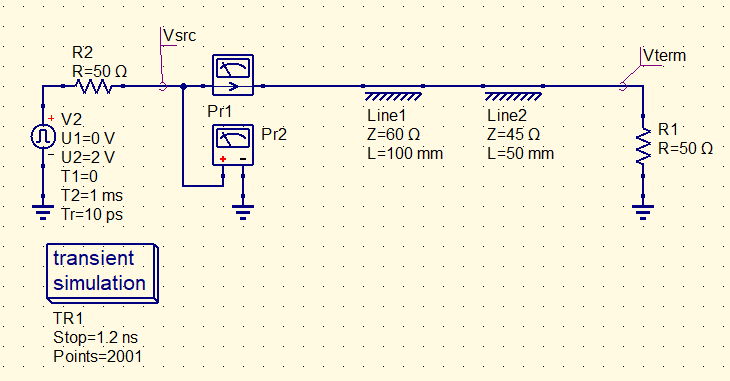
To see which is the impedance that the generator sees, you just need to measure its voltage and the current it drives. In the simulator you do this by adding two meters (Pr1, current and Pr2, voltage). You get the impedance by calculating the quotient of both.
Time domain response is as follows. You see how the impedance seen by the generator evolves across time. To get the evolution across distance, you need to know the signal propagation speed. The simulation (or a real measurement) allows to easily calculate the propagation speed as most of time the trace distance is a known factor.
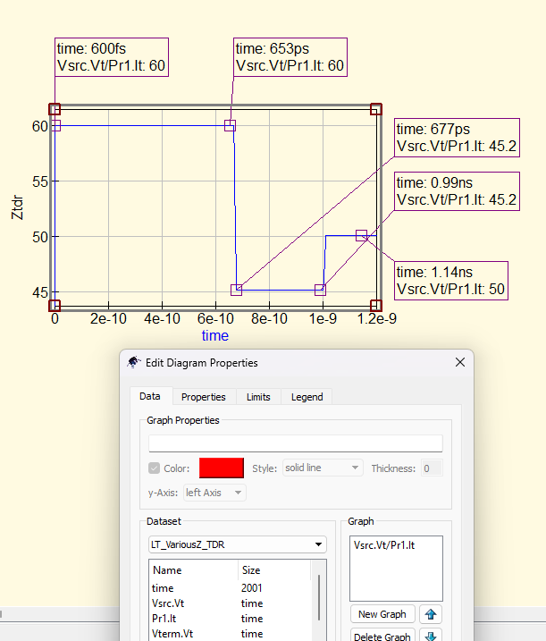
The time response is a very faithful reflect of the circuit except for the minor difference in impedance reported for the 45 Ω trace, which reflects a value which is 0.4 % higher. Where does this difference comes from? I do not know, since the termination resistor seem to give a perfect report: 50 Ω. Notice we are using ideal elements. My guessing is that there are rounding errors. When zooming the graph I see very small differences from ideal parameters. If someone has a reasonable hypothesis, do not hesitate to include a note in the newsletter comments.
Field simulator
With QucsStudio we could do a further thing that is not available in most circuit simulator: perform a 3D field simulation. Since it is possible, I have devoted long time and have used many alternative strategies, but I have failed in doing. Fernando suggested me to start from the different examples and do very minor modifications. In the examples that come with the simulator such simulation is possible.
Maybe we will have to wait for a new simulator revision.
Summary and conclusions
We have evaluated QucsStudio simulator. It is a powerful and user friendly tool but it is still under development. We have moved from pure ideal transmission line to others characterized by their mechanical/electrical properties. We have introduced in very summary way the s-parameters. We have solved some mysteries have been solved but others remain open.
Antoine de Saint-Exupéry author has seen a dragonfly crashing against his lamp when preparing to pilot a plane in Sahara desert. He knows it is the prelude of a sand storm. Then he writes: «This was not what excited me. What filled me with a barbaric joy was that I understood a murmured monosyllable of this secret language, had sniffed the air and known what was coming, like one of those primitive men to whom the future is revealed in such faint rustlings; it was that I had been able to read the anger of the desert in the beating wings of a dragonfly.» (Wind, Sand and Stars, Chapter 'Men of the Dessert', end of section II)