


QucsStudio evaluation and transmission line mismatch (1)
Evaluate a tool with a simple system that defies your understanding of things

Recently I have read a book from Antoine de Saint-Exupéry. The book was published in 1936 in English as 'Wind, Sand and Stars' and in Spanish as 'Tierra de los hombres'. A wonderful book full of human sensitivity, which I strongly recommend.
The back cover of the book in the Spanish edition says: «But what he (the author) really wants to tell us is that living is venturing out in search of the mystery hidden behind the surface of things, the possibility of finding the truth within oneself and the urgency of learning to love, the only way to survive this dehumanized universe». (Translation is mine)
Problem statement
When a transmission line is not terminated in a resistor equal to line's characteristic impedance you will observe reflections in the signal.
When you evaluate this system in the frequency domain, you will observe ripple in the transmission and reflection loss. There will be some frequencies in which the reflections will be destructive and the attenuation will grow and others in which the reflections will be constructive and attenuation will be lower.
This has a very practical implication when you have to measure any system whose characteristic impedance is different from 50 Ω single ended (or 100 Ω differential), as most1 measurement instrumentation is build over these 50 Ω. This is not as uncommon as you may think because there are may high speed transmission standards (PCIe, USB and others) that specify different characteristic impedance targets.
When the termination or the instrument Z0 and the cable have different impedances, you will observe some effects that may annoy you when you face it the first time. Al least, this happened to me the first time I came to this, and today I want to share with you some learnings I got.
For doing it, I am going to introduce a nice simulation tool: QucsStudio. This exercise of today will, at the same time, be used to evaluate it. There is nothing like evaluating tools with simple examples: this allows you to gain confidence of the program (no tool is perfect) while the example may also challenge our understanding of things.
It seems to me that those who complain of man's progress confuse ends with means. True, that man who struggles in the unique hope of material gain will harvest nothing worthwhile. But how can anyone conceive that the machine is an end? It is a tool. As much a tool as is the plough. The microscope is a tool. What disservice do we do the life of the spirit when we analyze the universe through a tool created by the science of optics, or seek to bring together those who love one another and are parted in space? (‘Wind, Sand and Stars’, chapter 3, The Tool)
QucsStudio
QucsStudio evolved from the QUCS project (link). This name stands for Quasi Universal Circuit Simulator. That was originally developed by Stefan Jahn and Michael Margraf among others. Its goal was to become a full electronic circuit simulator, including typical SPICE simulations (DC, AC, transient) and also those of RF design (S-parameters, Harmonic Balance). It used its own simulation engine, Qucsator, which is different from SPICE. It also has a very well designed graphical interface, based on Qt, which provides a very comfortable and effective user interface. Qucs latest public activity is related to 2017.
QucsStudio evolved from it and it is a reasonably active project. Latest version is 4.3.1, was released the 26th September 2022. It has been developed independently by Michael Margraf, and its binaries are available only for Windows. QucsStudio introduces a new simulation engine and adds unique features not present in the other variants such as system simulation, electromagnetic simulation of PCBs, or integration with C/C++, Octave and Kicad. Quite impressive but being a single man work may be slowing down a very ambitious and impressive development.
A very nice introduction to QucsStudio has done by my friend Fernando and if you want to go deeper in this wonderful tool, I encourage you to visit this link.
I have found in the tool some bugs and limitations, but despite this, I must say that while I continue evaluating it, I was surprised about its speed, intuitive operation and capabilities.
What does QucsStudio offers over other simulators like LTspice? Basically it is designed for RF circuits. As Signal Integrity and RF are brother disciplines, it is a very useful tool for me and I hope also for you. In few lines we will show it offers unique capabilities.
Create project in QucsStudio
To create a new project click over 'Projects' > 'New' > 'Create'.
It starts from 'Schematic'. Go to the 'Components' vertical tab and start adding components.
An ideal Transmission Line
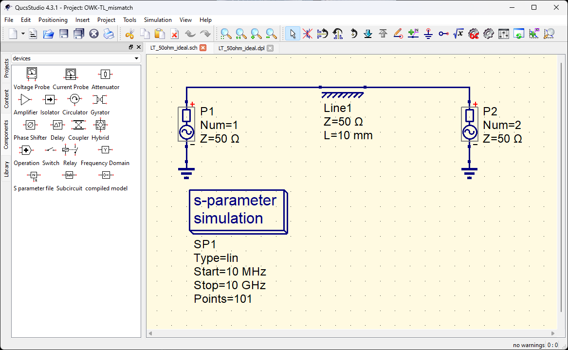
Let us start our project from ideal components. The first schematic includes:
voltage generator: we will select the vertical tab ‘Components’ and then ‘sources’ in the horizontal sliding menu. As we want to use s-parameter modeling, we will include ‘Power Source’ and not ‘ac Voltage Source’ which could be used for transient analysis for example.
transmission line: tab ‘transmission lines’ and select a ‘transmission line’.
simulation configuration: tab ‘simulations’.
ground connection, find it in ‘lumped components’ or in the taskbar.
The second step is to configure elements adequately. Select the component with the right mouse button and select ‘Edit Properties’ or double click over the component or directly place cursor text to change, click and type. Very intuitive.
For simulating, click over the gear or select ‘Simulate’ > ‘Simulation’ or F2.
Let us calculate impedance seen from the source, adding another cartesian plot. When editing properties, start typing the equation in ‘Graph Properties’ space. Searching over the help (or Fernado’s article) I found that exists an operator called rtoz(s,Z) that convert reflection coefficient with reference impedance to line impedance. It uses the following formula. I have tested both and the result is identical (as should be).

You may click over s-parameters lines to avoid typing them. In the properties tab, type ‘Z0 (Ohm)’ in the ‘left Axis Label’ parameter to make the figure more descriptive.

Placing markers are really intuitive and editing position simply superb.
In this plot we can see that the line really behaves as an ideal 50 Ω transmission line: return loss (s11) is negligible, infinite (-400 dB is very close to nothing). In summary, all energy is delivered to the load (s21), and nothing is reflected back to the source (s11).
“In the enthusiasm of our rapid mechanical conquests we have overlooked some things. We have perhaps driven men into the service of the machine, instead of building machinery for the service of man.” (‘Wind, sand an stars’, chapter 3, The tool)
The next week we will advance evaluating the tool with less ideal, more practical transmission line and we will approach to the understanding of basic things about s-parameters for Signal Integrity.
Broadcast systems have 75 Ω characteristic impedance and so it have its specific instrumentation.
What a great surprise! Thank you very much for sharing.