


Signal Integrity: when a serial source connection is a good option
And how simple simulations can save the day

In today’s post, I want to show how simple simulations can be used to complement back of the envelope calculations and concepts. For this, I will use real examples.

Some time ago, I had to develop a complex system which had an output that provides one pulse per second. Has a very sophisticated name: 1PPS. Try to guess why :-)
Such a signal, could ever had signal integrity problems? Remember that is slew rate what counts and not the signal period. And such a signal should have a reasonably fast slew rate because it is a synchronization one. The fastest the transition, the less the noise influence in the timing. Such a signal needs signal integrity considerations.
The equipment output had a BNC connector. In the most typical application, the user connects to it a coaxial cable of unknown length and the other end to the destination equipment. The termination is responsibility of the user.
In such application, serial source termination is an ideal solution because if the system is well matched in the source, despite the termination at the end, the final pulse will be a perfect replica of the original one.
Let us analyze it by simulation. We will use:
Ideal voltage pulse generator, with null internal impedance. In our example it is useless to complicate existence with more precise driver models. This could may make sense if we have to simulate an specific design.
Series resistance, equal to the cable characteristic impedance. In practice this resistance should to have a value such that the combination of the driver internal impedance and this resistor is as close as possible to cable Z0.
A lossless transmission line. Such model is characterized by just two parameters: delay time (Td) and characteristic impedance (Z0). SPICE has another model for lossy transmission lines that has a large number of parameters. For a system like ours, using it is put of scope.
The final termination. To make simulation more interesting we will use an .step directive to simulate different values in the same plot. Later on, I have manually added labels of the same color of the trace to make the result more clear.
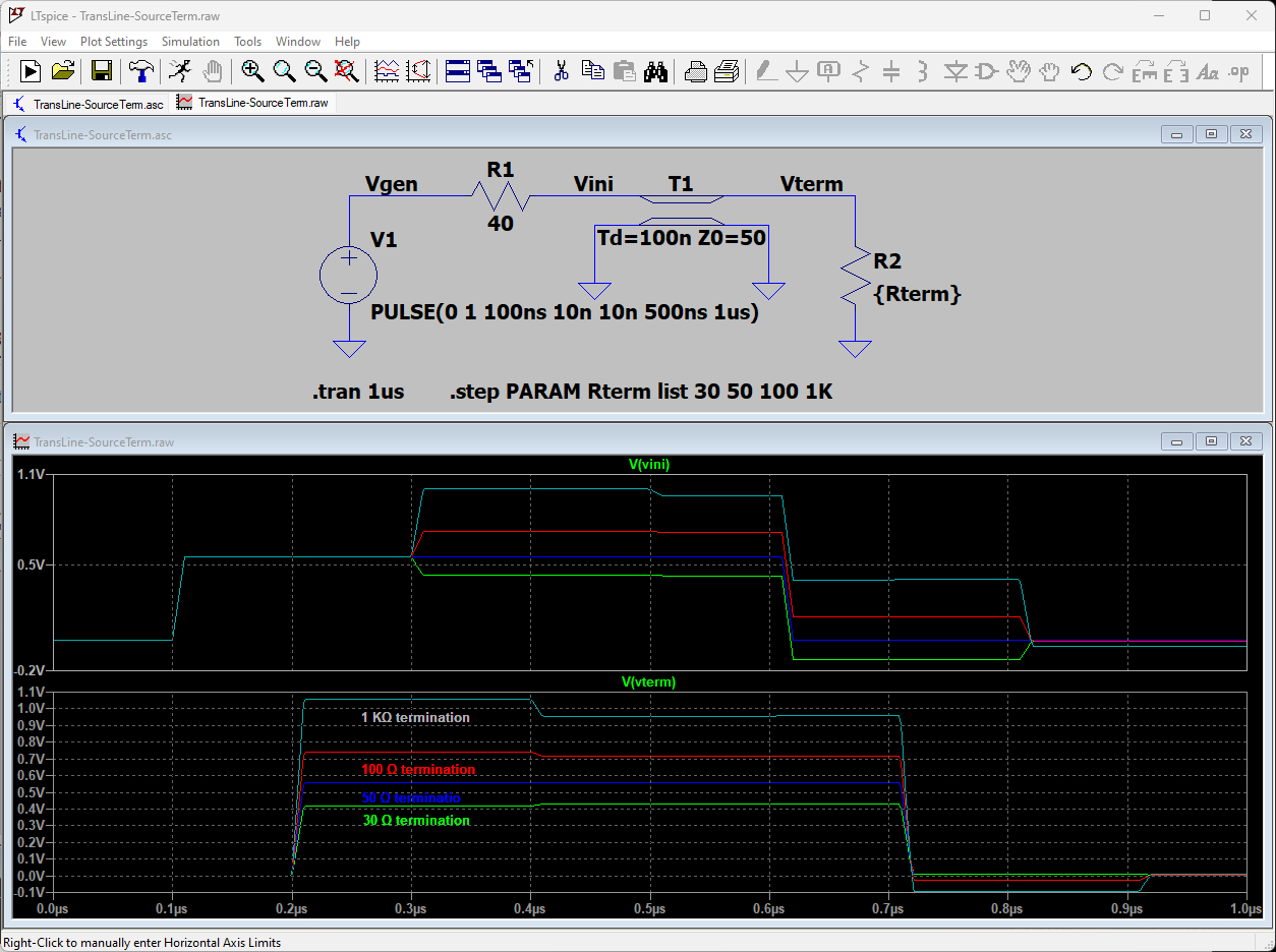
Follows the LTspice simulation screen. In the upper part we find the simulated circuit. In the central, the simulation plot of the voltage at the transmission line input (Vini) and in the lower part, at the output (Vterm). See the labels in the electrical diagram.

Eric Bogatin, a very capable Signal Integrity evangelist, used a very convenient image to understand signal integrity phenomenon. We propose to be the signal. This is why is portal is http://www.bethesignal.com. Following Eric's advice, we will surf over the signal :-)
The generator will see a 50 Ω resistor followed by a 50 Ω transmission line. Consequently, corresponding to 1.0 V step, it will drive 10 mA. Half of it will be the drop in the series resistor and half in the cable. This 0.5 V/10 mA step will start to propagate across the cable.
Remember we are the signal. After 100 ns (the transmission line delay, and arbritrary value I set) the edge reaches the destination. If it founds a 50 Ω load the 10 mA current of the generator makes an perfect mach and everything fits. If the resistor is lower, the voltage seen will be lower, if higher, higher. It is not the time to loose focus with the details, which are very easy to find in the literature. If the matching is not perfect, the current drained by the resistor will not be of the same amount that was flowing across the cable (50 mA). What happens is that part of the signal being reflected back to the source and starts a propagation in the opposite direction.
We will surf again over this reflected signal. When the edge reaches the origin, it finds a perfect match between the cable characteristic impedance and the load impedance. In this ideal model, reflections will stop.
If we concentrate in the voltage drop over R2 (Vterm), the termination voltage is always perfect: a delayed replica of the source and no pulse deformation. The only disadvantage of the source serial termination is that the received level is lower than the original: one half if matching is perfect in the source and in the end.
In the next figure we see what happens when the source matching is not perfect: when the reflected signal reaches the source there will be small reflections. This creates small distortion in the destination pulse.
The PPS circuit worked perfectly. The whole system was very complex but the devil is in the details and this small part had to be carefully cared.
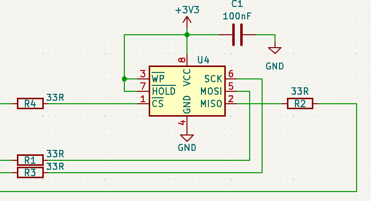
The series source termination is quite common in digital PCAs but used with some constraints. It is a good choice when there is point to point and unidirectional connections and typically there is no termination match to avoid the loss of signal level. It is very common to use 22 or 33 Ω resistors with no more considerations that this adds to driver internal impedance, which typically have some tens of Ohm.
For perfectionists: if we know the impedance of the transmission line and we measure with the oscilloscope the waveform after the series resistor, we can calculate the driver internal impedance. This could allow us to improve matching (and gain knowledge).