
Power Distribution Network - The devices (3)
Components and strategies we have to tame the power distribution network impedance.

Elements that influence the power network impedance
Overview
In a real circuit, what can we do to reduce PDN impedance?
If you analyze the impedance, you will find that it can be divided into regions, and within each region there is a single dominant factor. I have done the math and I was surprised to see how accurate this distribution by regions is:
Voltage regulator module (Power Supply Unit): DC to ~10 kHz
Bulk decoupling capacitors: ~10 kHz to ~200 kHz
SMD (MLCC) decoupling capacitors: ~200 kHz to 20 MHz. Do not expect MLCC to reduce PDN impedance above 50 MHz due to devices parasitic inductance.
On chip capacity: over 100 MHz
Let us study these elements in detail.
Voltage regulator module
Always expect the output impedance of a voltage regulator module (in every form) will have a high pass response like the one of next figure. It is very low at low frequency but rises at a 10 factor per decade (first order system).

We could see this from another point of view: never forget that a voltage regulator is a (negative) feedback system. The large open loop gain of the system has the effect to reduce the output impedance as far as this gain is higher than the feedback one. Reached this point, the output impedance will start to roll up.
We can see this from another point of view by means of an example. I have been recently working with ADP2116, which is a modern switching regulator. Next figure shows his response to a change of current load (also called Load Regulation). In the data sheet we can see that the load regulation is 0.03%/A. At 3 A, the voltage variation will be just 0.1%, 2.5 mV in my application. The output impedance at DC is 0.8 mΩ, which is extremely low.
However, in the transient we see a typical first order response: the reaction of the feedback system. The horizontal scale of the plot seems to be 400 μs/div. By naked sight, I could estimate a time constant of 100 μs, which is equivalent to a cutoff frequency of ~1.6 kHz. At that frequency the output impedance will start growing.

In summary, the power supply unit itself has a very low output impedance from DC to about few 10's of kHz.
Bulk decoupling capacitors
Bulk decoupling capacitors are those large value ones we place in the output of a Voltage Regulator Module.
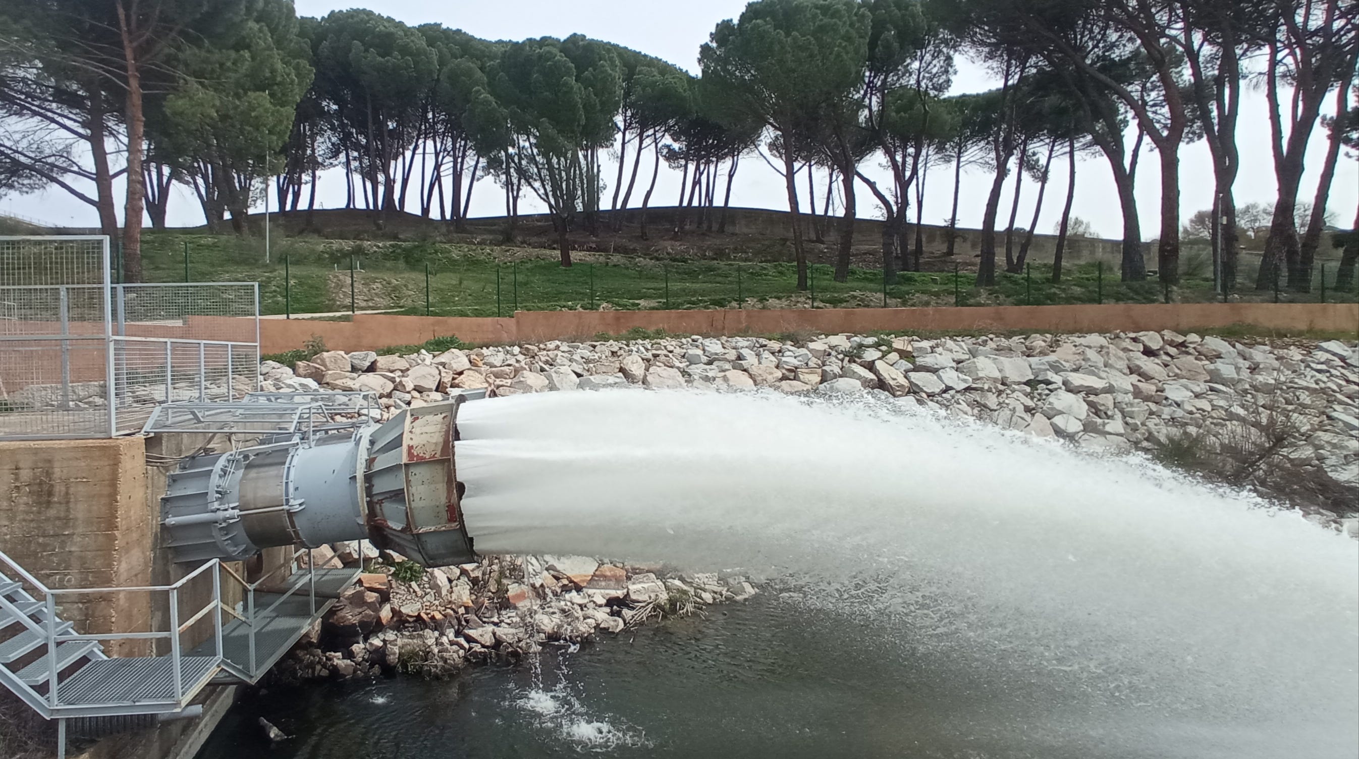
A good electrical model of an Aluminium Electrolytic capacitor is this composed of a series RLC circuitry. Have a look to next figure, valid for a 100 μF, 50 V, SMD and size of 10 x 10 x 10 mm. The data has been obtained from Wurth RedExpert.
This data is quite compatible with a series RLC model up to many hundreds of MHz with:
C=100 μF (the nominal value)
R=225 mΩ, also called ESR, Effective Series Resistance. This is a figure that it is typically provided by the capacitor manufacturer in its datasheet. It is very dependent on physical parameters. The bigger the size of the capacitor is, the lower it will be.
L= 5.3 nH. Typically not published by manufacturers. In this particular example, the inductance becomes dominant at few units of MHz.
There are other technologies like aluminum polymer that offer lower ESR and inductance, although at a higher cost and lower voltage.
For decoupling of switched mode regulators, it is very important that the capacitor behaves dominantly as a capacitor even at ten times the switching frequency. If this cannot be done with bulk electrolytic capacitors, it may happen that you can use ceramic capacitors of lower capacity in parallel. They have much lower ESR values than electrolytic ones as we will see just now.
However, for PDN engineering is just the impedance what counts.
Multilayer Ceramic Capacitor (MLCC)
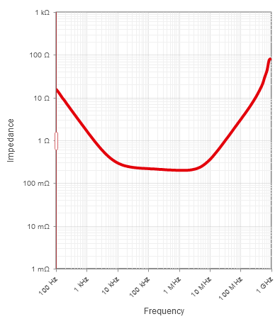
Let us use Wurth RedExpert once again to obtain data from a common use capacitor. This time will be a 1 μF, 50 V, X7R, with case 0805.
In this time, the parameters of the RLC model are:
C=1 μF (the nominal value, 100 times less than the previous one).
R=5.3 mΩ ESR. It is ~40 times less than the previous one. It is also dependent in case and voltage (the higher ones, the lower ESR).
L= 283 pH. This is ~20 times less than the previous one. The circuit resonates a about 10 MHz.
The net figure shows the impedance measurement of various capacitors of different technologies and sizes. This shows clearly show that cleverly placing various capacitors in parallel, we can optimize the impedance seen by the load.

It is very nice that RedExpert provide in table format the three values of the series model and also the impedance in graph format, among other information.
During decades the advice has been to place one 100 nF ceramic capacitor close to IC supply pins and one larger value (10 or 100 times more) very 10 power pins. Now, you can understand where this advice comes from. It is a generic rule of thumb but a very reasonable rule of thumb.
However, today the suggestion is to place the maximum X7R capacitor that you can find for the allowable room. My experience is that 1 μF MLCC can be a right capacity value for most but the most stringent space boards.
In next post we will continue the analysis seen what happens in the circuit because not only the components have influence in the performance. Beware of inductance as much as the Ides of March :-)