

Measuring distortion
Measuring distortion
A story of lines, curves and tones

Some years ago I had to work in the design and characterization of a high bandwidth optical LED driver. The optoelectronic device was far from being linear: reaching a certain point as driving current increases, the output light level does not grow in the same proportion. This property is not specific of optical devices: many RF power amplifiers are operated in regions in which linearity is far from being perfect. Digital techniques of predistortion or distortion compensation may lead to amazing results but the first step is always the open loop characterization of the system.

Photo by Lisa Yount on Unsplash
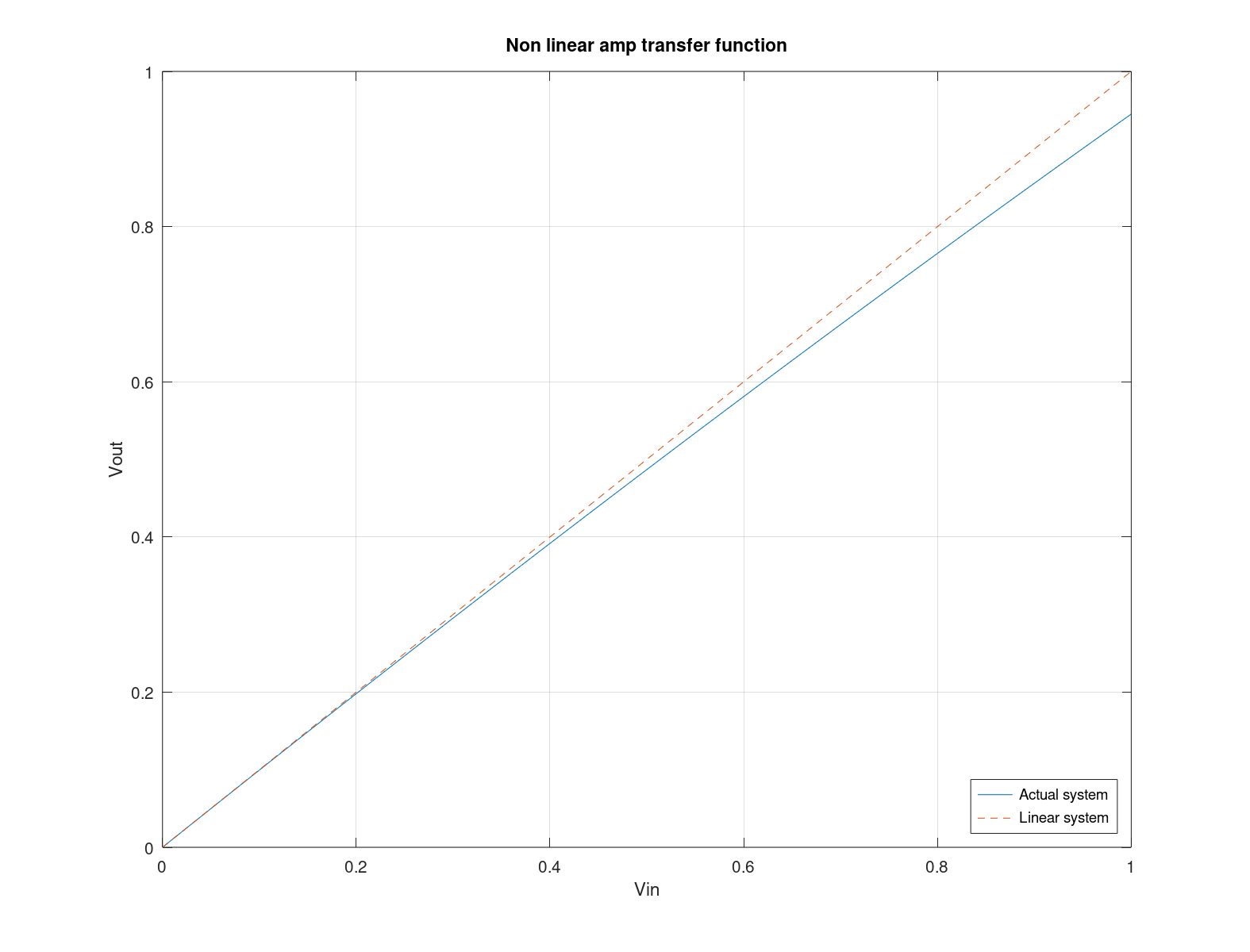
Let us show the behavior in a simulated system. The figure shows the transfer function of an ideal system (in dotted line) and a simulated one (continuous blue line).
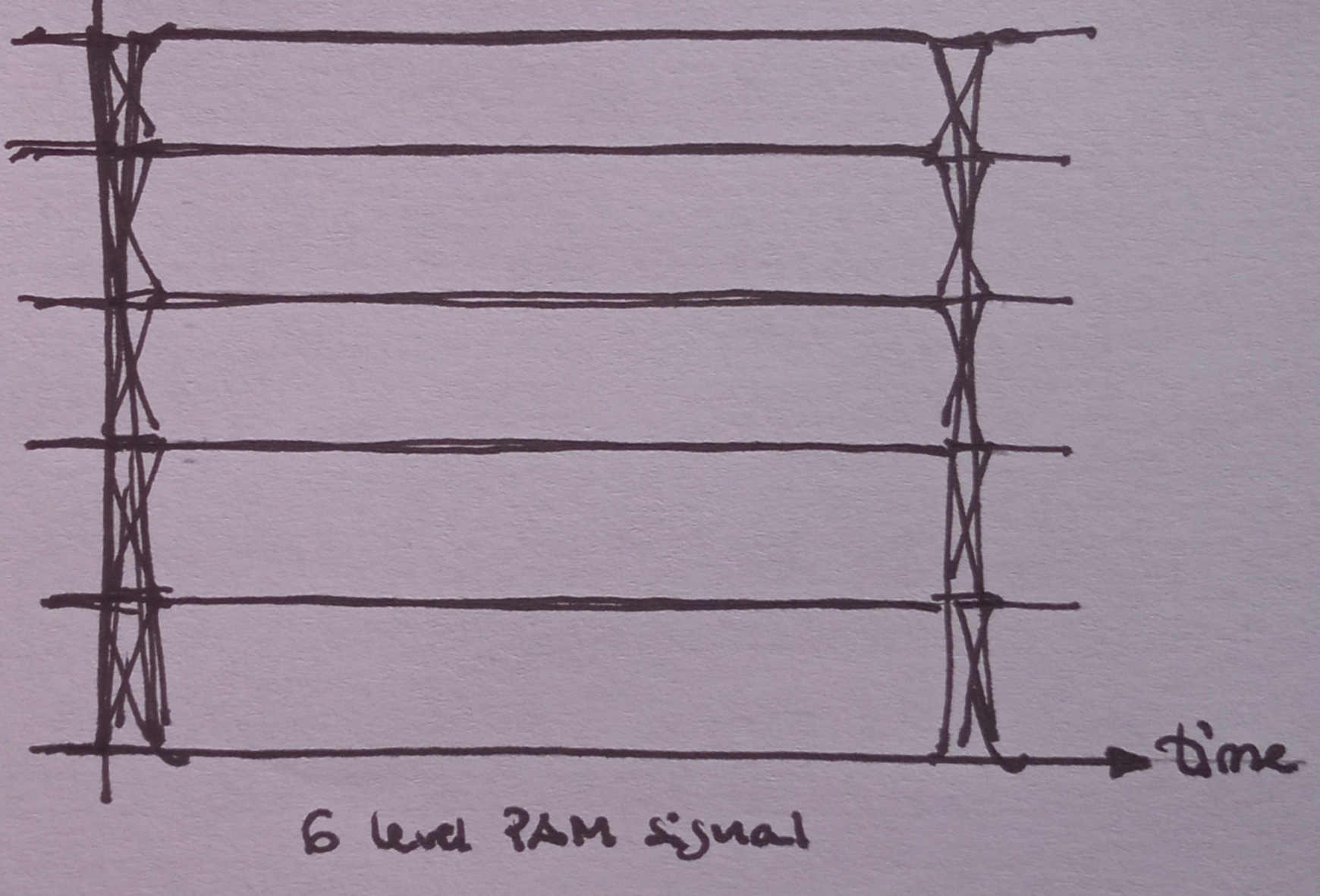
Because of that, when we transmitted a various level PAM (Pulse Amplitude Modulation) digital signal, the compression at higher signal level was clearly visible.
When dealing with non-linear systems we need to be very careful. We engineers have studied Linear Time Invariant (LTI) systems. Non linearity is terra incognita and tends to be difficult to deal with. For example, strictly speaking, a non-linear system has not a frequency response. If non-linearity is low, we can still use the concepts of linear systems… with care. But no one will tell you the type of things you have to care of :-)
While the task of measuring distortion looked simple, it proved to be a very complex and appealing challenge.
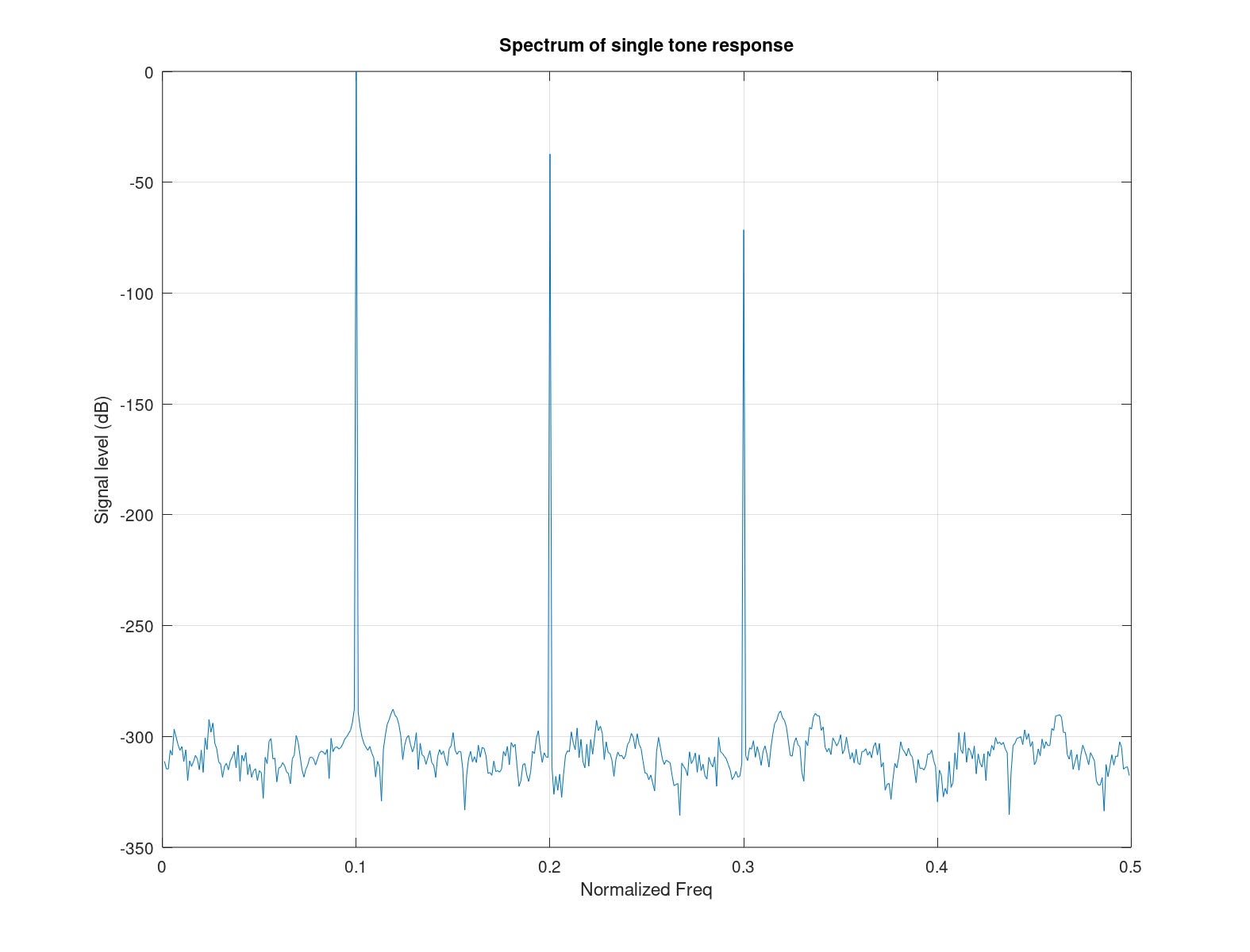
The most classical way we have to measure distortion is to inject a pure tone at the input of the system and to measure harmonics at the output with an spectrum analyzer (SA). Worth remembering that a system which has symmetrical amplitude response (say a saturating transformer) has no even harmonics at its output, but this is not our case because an optical system is intrinsically asymetrical: the negative light does not exist. If the input tone frequency is f1, we were able to measure significant components at 2·f1 and 3·f1 . Higher harmonics were negligible.
Later on we discovered (in the hard way) that we had to be very careful with harmonic content of the generator itself. We used an old synthesized RF generator. Its second harmonic was about -50 dBc. [You may be unfamiliar with the dBc expression: means dB over carrier]. We solved the problem of the generator distortion by using SMA male to SMA female low pass filters from Minicircuits. Great devices.
We also found that what lecture books says about harmonic level is essentially true. Imagine you are far from compression point (in practice, this is true for any usable signal level). At that point, if you increase the input level by n dB, the output fundamental frequency increases by n dB. So far, as expected. The first harmonic (2⋅f1) increases by 2n dB and the third harmonic (3⋅f1) by 3n dB. This rule, that does not take into account the actual distortion mechanism, has quite good prediction capability.
At that point, we had also to deal with a fact: while the current to light converter device was expected to have similar distortion behavior with frequency, the driver has not by no means. This would require a full article, but in summary we could say that the amplifiers we build are quite non linear devices that behave linearly thanks to he fact we apply large amounts of negative feedback. Because of that it is reasonable to think that as open loop gain decreases at high frequency, the beneficial effects of feedback decreases. This turned out to be true.
This means that to fully characterize the system, we have to measure distortion not only at low frequency but also at high frequency. And at that point another disturbing effect appeared. As I increased the frequency of the measurement tone, I saw that the harmonic level decreased, exactly the opposite of the expected. The reason for that is easy to understand: the bandwidth limitation of the system attenuates the high frequency harmonics. But this does not mean that the distortion is reducing: what reduces is the way we have to characterize it! This was bad news because the measurements revealed a situation that is more optimistic than reality.
Said in other words: the measurement technique was revealing its own limitations. And the limitation is strong because as we increase the frequency, the harmonics frequencies are increasing at a higher rate. If we measure at 1 MHz, harmonics are at 2 and 3 MHz. If we measure at 10 MHz, there were 20 and 30 MHz still inside bandwidth. But if I measure at 50 MHz the signal was inside the usable bandwidth but harmonics are definitively not.
Fortunately, there is another classical way to characterize distortion: using two tones and measuring the intermodulation tones. The input signal is the combination of two tones of identical amplitude and different frequencies: f1 and f2 . At the output you are going to get harmonics whose frequencies are n⋅f1 ± m⋅f2 . The best idea is to use frequencies that are close between them.
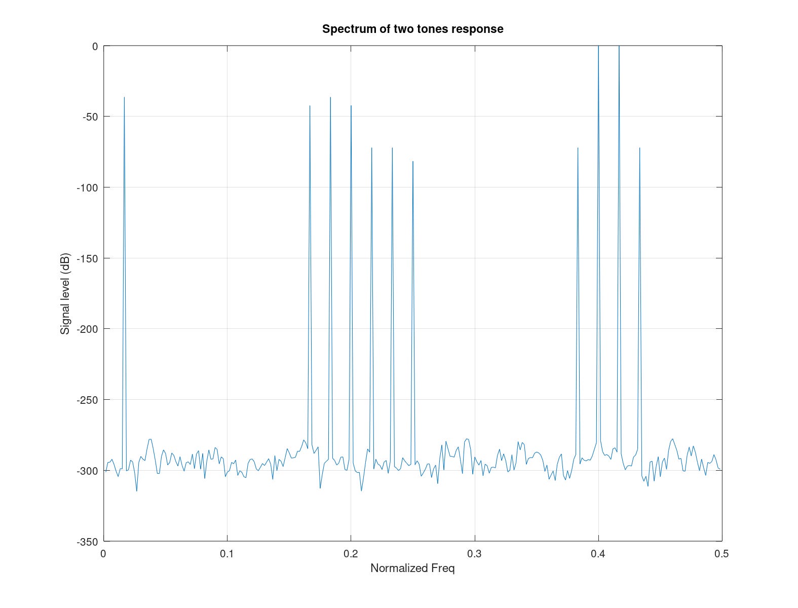
The magic of this technique is that the intermodulation tones you have to measure can be very close to the stimulus tones and you can avoid the restriction of the system bandwidth.
At that point, the tones we injected did not came from a RF generator but from a DAC. Its internal distortion level was very good. We adjusted level to have a peak signal of -1 dB of full scale.
Follows the Octave/Matlab code used to generate the post images. There is a main file and two functions.
% Support file for 'Measuring distortion' post
% ---------------------------------------------------
close all;
clear;

gain= 1;
sec_ord_factor= -0.05;
NoT= 100; % Number of tone periods

% Non linear device transfer function (Vin -> Vout)
% ---------------------------------------------------
Vin= 0:0.01:1;
Vout= non_lin_amp(Vin, gain, sec_ord_factor);
figure(1);
plot(Vin, Vout, [0 1], gain*[0 1], '--'); grid on;
xlabel("Vin");
ylabel("Vout");
legend("Actual system", "Linear system", "location", "southeast");
title("Non linear amp transfer function");

orient('landscape');
print('-dpdf', "trasns_funct.pdf");
print('-dpng', 'bestfit', "trasns_funct.png");

% Response to one tone
% ----------------------------------
F1_norm= 0.1;
NoTP= ceil(NoT/F1_norm);
t= 1:NoTP;
Vi= 0.5 + 0.45*cos(2*pi*F1_norm*t);
Vo= non_lin_amp(Vi, gain, sec_ord_factor);

display_spectrum(Vi, "single tone");
display_spectrum(Vo, "single tone response");

% Response to two tones
% ----------------------------------
F1_norm= 0.40;
F2_norm= 1/2.4;
NoTP= ceil(NoT/(F1_norm*F2_norm)); % Number of time points: integer numer of periods

t= 1:NoTP;
Vi= 0.5 + 0.25*(cos(2*pi*F1_norm*t) + cos(2*pi*F2_norm*t));
Vo= non_lin_amp(Vi, gain, sec_ord_factor);

display_spectrum(Vi, "two tones");
display_spectrum(Vo, "two tones response");
% non_lin_amp: time response model of a generic and invented non linear amplifier
% ------------------------------------------------------------
% Input:
% - Vin: input signal in time domain
% - gain: gain of the reference linear system
% - second_order_term: coefficient of the second order polynomial
%
% Output:
% - Vout: amplifier output signal in time domain
%
function Vout = non_lin_amp (Vin, gain, sec_ord_term)
if (nargin < 2)
gain= 1;
endif
if (nargin < 3)
sec_ord_term= -0.1;
endif
if (nargin < 4)
third_ord_term= -0.005;
endif
Vout= gain*Vin + sec_ord_term*Vin.^2 + third_ord_term*Vin.^3;
endfunction% display_spectrum - Displays the spectrum of a signal and generates file plot
% ---------------------------------------------------
% Input:
% - signal: time domain signal
% - descrip_txt: string usef for file name suffix
function display_spectrum (signal, descrip_txt)
spect= abs(fft(signal));
spect_dB= 20*log10(spect);
spect_dB= spect_dB - max(spect_dB(2:end-1));
frq_norm= 0:1/length(signal):1;
inx= 2:floor(length(signal)/2);
figure();
plot(frq_norm(inx), spect_dB(inx)); grid on;
ax= axis();
ax(2)= 0.5;
axis(ax);
xlabel("Normalized Freq");
ylabel("Signal level (dB)");
title(sprintf("Spectrum of %s", descrip_txt));
orient('landscape');
fn= sprintf("spectrum-%s.pdf", descrip_txt);
print('-dpdf', fn);
fn= sprintf("spectrum-%s.png", descrip_txt);
print('-dpng', 'bestfit', fn);
endfunction