

It looks high speed but, is it really high speed?
It looks high speed but, is it really high speed?
Real examples of lumped vs transmission line circuitry


Today we are going to examine three examples of real lumped vs transmission line circuits.
I2C interface
I2C is a serial bus that operates at 400 kbps maximum and should not produce Signal Integrity issues, wright? Wrong!
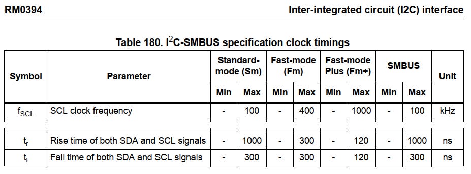
Once I was debugging a board with an STM32 ARM MCU manufactured by ST and was able to measure a 2.9 ns falling edge. Follows a picture the manufacturer’s specifications. You will be able to see in it that only the maximum values are provided. From this side we cannot advance more.
The spacial extend of an edge over a microstrip line over FR4 of the (measured) I2C falling edge is
We will have to apply Signal Integrity considerations if trace length is longer that one sixth: 80 mm.
A comment is required at that point: I2C FAST mode works at a maximum rate of 400 kHz. A bit time takes 2.5 μs to transmit. Fall time does not need to be that fast: the measured value is 1/1000 of bit time. The designer has various complimentary approaches: configuring port by FW for slower slew rate and/or to slow it down by hardware by adding a carefully chosen series resistor and a capacitor. This will move the Signal Integrity care to much longer distances.
Fast LVDS lines
Let us consider a system that uses uses LVDS (Low Voltage Differential Signalling) and uses the MAX9112 TTL to LVDS driver. The data sheet reveals RT/FT is between 0.25 to 1 ns.

Let us imagine our system uses 1.27 mm ribbon cable. The manufacturer reports a propagation delay of 4.3 ns/m (which is equal to 4.3 ps/mm).
We will have to apply Signal Integrity considerations if trace length is longer that 10 mm. Almost every system will be longer. LVDS drivers tend to be very fast.
CAN bus interface at 1 Mbps
CAN bus is widely used in automotive and industrial machines among other systems. Let us consider the maximum data rate of the basic standard: 1 Mbps. One bit period takes 1 μs. As a rule of thumb, let us assign 1/10 of the bit period to the edges: 100 ns for Rise Time (RT) or Fall Time (FT).
The cable should be a 120 Ω differential characteristic impedance. I have found one with a propagation delay of 4.1 ns/m.
We will have to apply Signal Integrity considerations if cable length is longer that 4 m.
Someone could argue that the slew rate should be the one of the driver and not related to bit rate. This argument strongly depends on the design stage we are. If we are doing back of the envelope calculations while we are evaluating the architecture, actual calculation is reasonable. If we are evaluating a particular design in development, we may apply different approaches, from slew control of the driver itself (like MCP2551) or by controlling slew in our circuit. By the way: CAN driver manufacturers tend not to specify slew rate.
Another use of spacial extend of an edge
Having the figure of the spacial extend of an edge has another useful usage: you can use it to know if a disturbance is relevant or not in terms of signal integrity.
Any loss of uniformity like connectors or IC connections (both the visible one and the invisible inside the package) should be compared to the spacial extend of an edge. If this discontinuity is much less that 1/6 of it, can be considered negligible, but if bigger, the signal will perceive as discontinuity and there will be reflections.
Summary
Today we have seen:
Signal integrity considerations are not related to data rate but to slew rate of the signals. We may have margin to tune them and reduce SI problems.
Calculating the spacial extend of the edge of a signal is the primary calculation to orientate in the SI jungle.