


When I received some time ago the assignment of designing the air cooling of an industrial machine, I could not imagine how much problems I was going to have when estimating the worst case power needed to drive the fans. They are wild devices and if you have to deal with them is better to know how to navigate these windy waters. If I knew at that time the content of this post, my life would have been much easier.

Photo by Marius Matuschzik on Unsplash
First of all we have understand the most basic underlying physics.
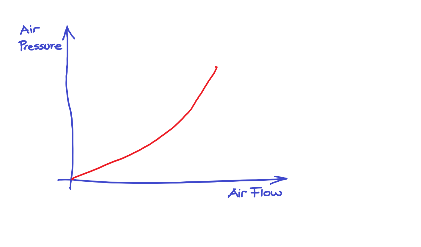
The graph below shows the relationship that rules the movement of air. In the horizontal axis we have the air flow (air volume per time unit) and in vertical axis the air pressure. If we want double air flow, we need to increase the air pressure a by a bit more than two times, in order to compensate for the turbulence of the flow. [If flow is laminar, the relationship is quite linear, but it it has many turbulences follows a pure square relationship (P=K·Q^2)].
Let us see now the graph that rules a fan.

Point A is the one you have if you place the fan in the middle of a room hanged from the ceiling with a wire. The pressure of the air is nearly zero (there is the same pressure at both sides of the fan) and the air flow is large.
Point B happens when the fan is is connected to closed box. As the box is closed, net air flow across the fan is null but due to the fan activity, the pressure of the air at the two sides of the fan is different.
Neither point A not point B are practical operating points. Normal operation of the fan is somewhere in between. The fact that the curve is very unlinear make things more funny but does not change things in essence. When the fan is placed in your system the two curves intersect like in the figure below.

So far all the explanation is for a fan whose is speed is maximum. If fan speed can be electronically controlled, we get the following figure.

So far, fan generic behavior. Now, let us move to the world of real devices, and let us use a nice fan, part number 4114 N/2H7P from Embpapst, a high quality German manufacturer. Link to the device page. This fan has electronic speed control based on a TTL level PWM signal and also has an open collector output with tachomenter pulses, whose frequency is proportional to rotation speed. This signal is very useful for device supervision.
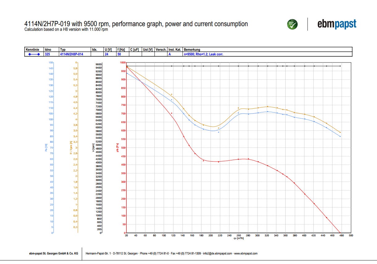
Next figure shows the device specifications. They need to be read with great care because power consumption figure (90 W) is for fan operating in point A in the previous figure.

The next figure shows the fan flow specification. The fan works optimally in the gray shaded area.

When you are dealing with fans and you have the graph of next figure you can consider yourself a very fortunate person, because it contains a lot of information. Among other, the worst case power demand you may have. The power is displayed in blue color and you can see that is a bit less that the specified 90 W for zero pressure but can reach 140 W for maximum pressure (and no air flow). That's 55 % more power. Consequently the power supply of this fan has to be dimension for this worst case plus a 10% extra margin. Depends on your system if this worst case can be reached or not.
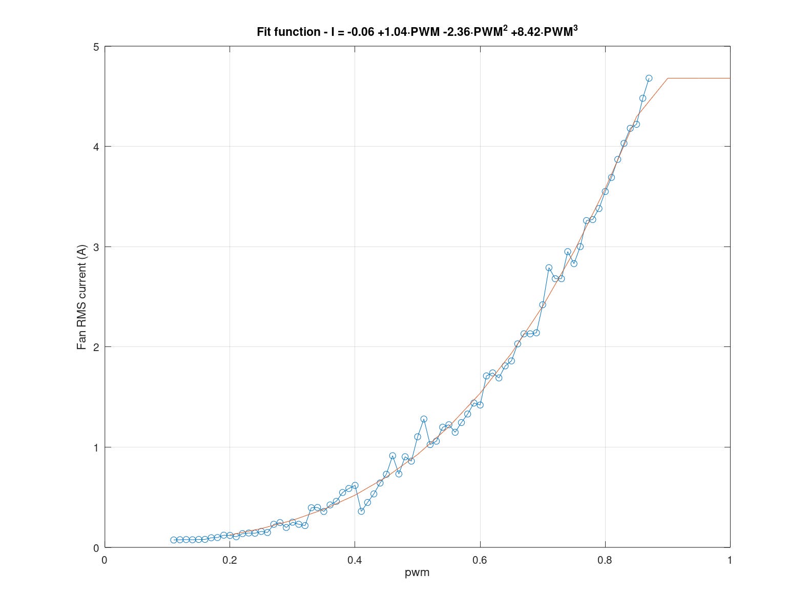
Just to finish, worth noticing that the current consumption of the fan follows a polynomial relationship, typically cubic. Maximum current is coherent to specifications because the maximum practicable control is a PWM of 0.85. Beyond this value, the control saturate and rotation speed does not increase more.
With this all information in your toolbox, you will be prepared to deal with the most dangerous missions that may involve fan power supply.